Graphic options for illustrating where Americans moved during COVID-19

I appreciate the effort at CityLab to take all of the data regarding where Americans moved during the COVID-19 pandemic and put it into graphs and charts. Good graphs and charts should help illustrate relationships between variables and help readers see patterns. Here are several choices that I thought succeeded.

First, start with patterns in metro areas across the United States.

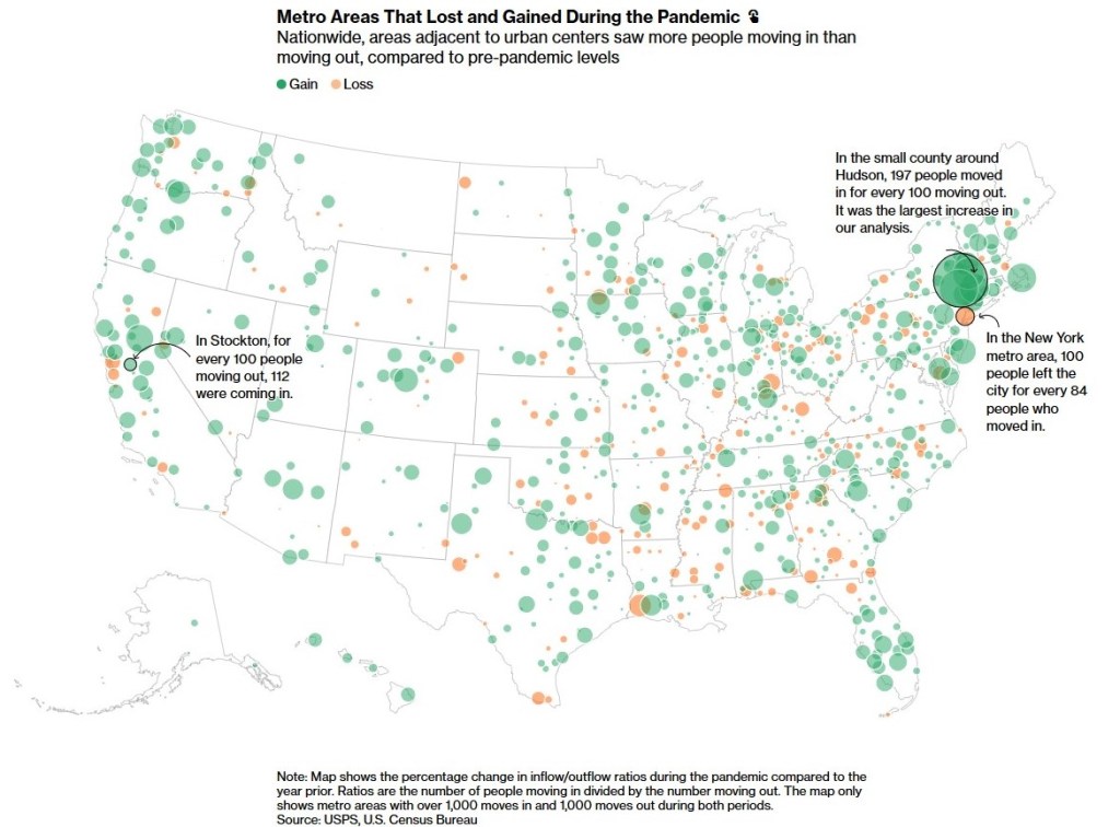
The two colors plus the size of the circle show the percentage change in population. The percentage is a nice touch yet the comparison to the previous year might slip past some viewers.

Second, another way to look at metro areas on the whole regarding population changes.

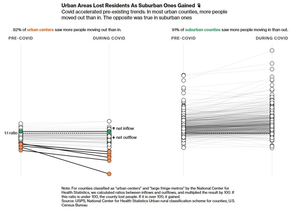
The side-by-side of central cities and suburbs quickly shows several differences: lower ratios for cities, more variability among suburban counties, more losses for cities during COVID. The patterns among suburban counties are a little hard to pick up; there are a number of counties that lost people even as the general trend might have been up.

Third, where did all those people moving from New York City, specifically Manhattan go?

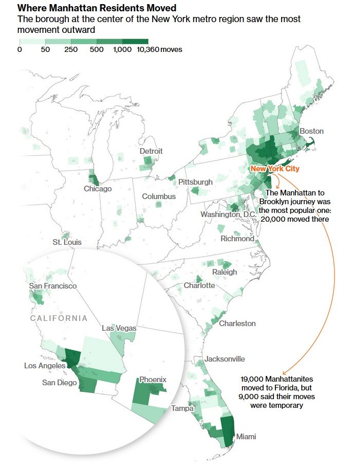
In absolute numbers, there are patterns this map displays nicely: a lot of moves in New York City and in the region plus moves to other metro areas (including Miami, Los Angeles, Chicago, and more). The inset of the Southwest at the bottom left is a nice touch…presumably New Yorkers did not move in large numbers to anywhere roughly between Nashville and Seattle.

Fourth, which New Yorkers moved?

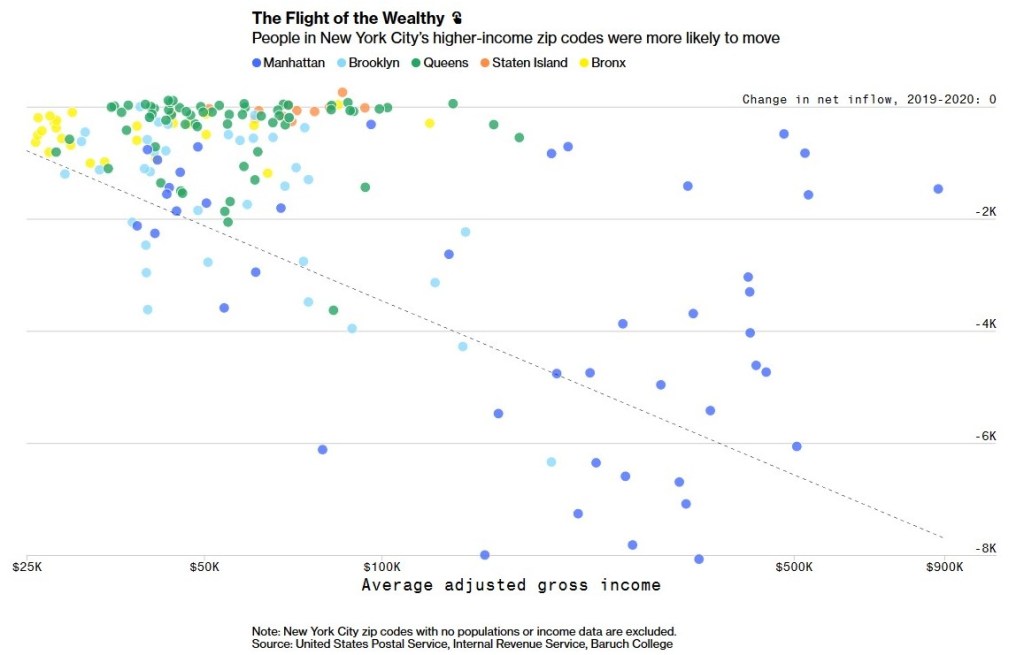
Looking at zip codes, neighborhoods with higher incomes had more people moving while the numerous neighborhoods with lower incomes had smaller changes in inflow.

All together, this is more than just a series of pretty graphics. These choices – first about what data to use and second about how to present one variable in light of another – help clarify what happened in the last year. Each choice could have been a little different; emphasize a different part of the data or another variable, choose another graphic option. Yet, while there is certainly more to untangle about mobility, cities and suburbs, and COVID-19, these images help us start making sense of complex phenomena.

When a pie chart works for analyzing the lyrics of a song, Hey Jude edition

Earlier this week, a data visualization expert presented a pie chart for the lyrics of The Beatles’ hit “Hey Jude”:

HeyJudeLyricsPieChart

Pie charts are very effective when you want to show the readers that a large percentage of what you are examining is made of one or two categories. In contrast, too many categories or not a clear larger category can render a pie chart less useful. In this case, the word/lyrics “na” makes up 40% of the song “Hey Jude.” In contrast, the words in the song’s title – “hey” and “Jude” – comprise 14% of the song and “all other words” – the song has three verses (the fourth one repeats the first verse) and two bridges – account for 40%.

This should lead to questions about what made this song such a hit. Singing “na” over and over again leads to a number one hit and a song played countless time on radio? The lyrics Paul McCartney wrote out in the studio sold for over $900,000 though there are no written “na”s on that piece of paper. Of course, the song was written and performed by the Beatles, a musical and sociological phenomena if there ever was one, and the song is a hopeful as Paul aimed to reassure John Lennon’s son Julian. Could the song stand on its own as a 3 minute single (and these first minutes contain few “na”s)? These words are still hopeful and the way the Beatles stack instruments and harmonies from a relatively quiet first verse through the second bridge is interesting. Yet, the “na”s at the end make the song unique, not just for the number of them (roughly minutes before fading out) but the spirit in which they are offered (big sound plus Paul improvising over the top).

Thus, the pie graph above does a good job. It points out the lyrical peculiarities of this hit song and hints at deeper questions about the Beatles, music, and what makes songs and cultural products popular.

Reminder: do not get carried away making fancy charts and graphs

The Brewster Rockit: Space Guy! comic strip from last Sunday makes an important point about designing charts and graphs: don’t get carried away.

https://www.gocomics.com/brewsterrockit/2020/05/03

Brewster Rockit May 3, 2020

The goal of using a chart or graph is to distill the information behind it into an easy-to-read format for making a quick point. A reader’s eye is drawn to a chart or graph and it should be easy to figure out the point the graphic is making.

If the graph or chart is too complicated, it loses its potency. If it looks great or clever but cannot help the reader interpret the data correctly, it is not very useful. If the researcher spends a lot of time tweaking the graphic to really make it eye-popping, it may not be worth it compared to simply getting the point across.

In sum: graphs and charts can be fun. They can break up long text and data tables. They can focus attention on an important data point or relationship. At the same time, they can get too complicated and become a time suck both for the producer of the graphic and those trying to figure them out.

Summarizing data visualization errors

Check out this good quick overview of visualization errors – here are a few good moments:

Everything is relative. You can’t say a town is more dangerous than another because the first one had two robberies and the other only had one. What if the first town has 1,000 times the population that of the first? It is often more useful to think in terms of percentages and rates rather than absolutes and totals…

It’s easy to cherrypick dates and timeframes to fit a specific narrative. So consider history, what usually happens, and proper baselines to compare against…

When you see a three-dimensional chart that is three dimensions for no good reason, question the data, the chart, the maker, and everything based on the chart.

In summary: data visualizations can be very useful for highlighting a particular pattern but they can also be altered to advance an incorrect point. I always wonder with these examples of misleading visualizations whether the maker intentionally made the change to advance their point or whether there was a lack of knowledge about how to do good data analysis. Of course, this issue could arise with any data analysis as there are right and wrong ways to interpret and present data.

“The most misleading charts of 2015, fixed”

Here are some improved charts first put forward by politicians, advocacy groups, and the media in 2015.

I’m not sure exactly how they picked “the most misleading charts” (is there bias in this selection?) but it is interesting that several involve a misleading y-axis. I’m not sure that I would count the last example as a misleading chart since it involves a definition issue before getting to the chart.

And what is the purpose of the original, poorly done graphics? Changing the presentation of the data provides evidence for a particular viewpoint. Change the graphic depiction of the data and another story could be told. Unfortunately, it is actions like these that tend to cast doubt on the use of data for making public arguments – the data is simply too easy to manipulate so why rely on data at all? Of course, that assumes people look closely at the chart and the data source and know what questions to ask…

“New Apps Instantly Convert Spreadsheets Into Something Actually Readable”

Several new apps transform spreadsheet data into a chart or graph without having to spend much or any time with the raw data:

It’s called Project Elastic, and he unveiled the thing this fall at a conference run by his company, Tableau. The Seattle-based company has been massively successful selling software that helps big businesses “visualize” the massive amount of online data they generate—transform all those words and numbers into charts and graphics their data scientists can more readily digest—but Project Elastic is something different. It’s not meant for big businesses. It’s meant for everyone.

The idea is that, when someone emails a spreadsheet to your iPad, the app will open it up—but not as a series of rows and columns. It will open the thing as chart or graph, and with a swipe of the finger, you can reformat the data into a new chart or graph. The hope is that this will make is easier for anyone to read a digital spreadsheet—an age-old computer creation that’s still looks like Greek to so many people. “We think that seeing and understanding your data is a human right,” says Story, the Tableau vice president in charge of the project.

And Story isn’t the only one. A startup called ChartCube has developed a similar tool that can turn raw data into easy-to-understand charts and graphs, and just this week, the new-age publishing outfit Medium released a tool called Charted that can visualize data in similar ways. So many companies aim to democratize access to online data, but for all the different data analysis tool out on the market, this is still the domain of experts—people schooled in the art of data analysis. These projects aim to put the democracy in democratize.

Two quick thoughts:

1. I understand the impulse to create charts and graphs that communicate patterns. Yet, such devices are not infallible in themselves. I would suggest we need more education in interpreting and using the information from infographics. Additionally, this might be a temporary solution but wouldn’t it be better in the long run if more people know how to read and use a spreadsheet?

2. Interesting quote: “We think that seeing and understanding your data is a human right.” I have a right to data or to the graphing and charting of my data? This adds to a collection of voices arguing for a human right to information and data.

Adding a chart to scientific findings makes it more persuasive

A new research study suggests charts of data are more persuasive compared to just text:

Then for a randomly selected subsample, the researchers supplemented the description of the drug trial with a simple chart. But here’s the kicker: That chart contained no new information; it simply repeated the information in the original vignette, with a tall bar illustrating that 87 percent of the control group had the illness, and a shorter bar showing that that number fell to 47 percent for those who took the drug.

But taking the same information and also showing it as a chart made it enormously more persuasive, raising the proportion who believed in the efficacy of the drug to 97 percent from 68 percent. If the researchers are correct, the following chart should persuade you of their finding.

What makes simple charts so persuasive? It isn’t because they make the information more memorable — 30 minutes after reading about the drug trials, those who saw the charts were not much more likely to recall the results than those who had just read the description. Rather, the researchers conjecture, charts offer the veneer of science. And indeed, the tendency to find the charts more persuasive was strongest among those who agreed with the statement “I believe in science.”

Charts = science? If veneer of science is the answer, why does the chart support science? Scientists are the ones who use charts? Or they are the ones who are trusted more with charts?

I wonder if there are other explanations:

1. Seeing a clear difference in bars (87% vs. 47%) makes a stronger impression than simply reading the difference. A 40% difference is abstract but is more striking in an image.

2. More people accept the power of visual data today compared to written text. Think of all those Internet infographics with interesting information.

Strong spurious correlations enhanced in appearance with mismatched dual axes

I stumbled across a potentially fascinating website titled Spurious Correlations that looks at relationships between odd variables. Here are two examples:

According to the site, both of these pairs have correlations higher than 0.94. In other words, very strong.

One issue: using dual axes can throw things off. The bottom chart above shows a negative relationship – but this is only because the axes are different. The top chart makes it look like the lines really go together – but the axes are way off from each other with the left side ranging from 29-34 and the right side ranging from 300-900. Overall, the charts reinforce the strong correlations between the two variables but using dual axes can be misleading.

Evaluating the charts and graphics in President Obama’s “enhanced experience” version of the State of the Union

In addition to the speech, President Obama’s State of the Union involved an “enhanced experience” with plenty of charts and graphics. Here are some thoughts about how well this data and information was presented:

But sometimes, even accuracy can be misleading, especially when it comes to graphics and charts. On Tuesday night, President Obama gave his State of the Union address and the White House launched an “enhanced” experience, a multimedia display with video, 107 slides and 27 charts…

Overall, Few said Obama’s team created well-designed charts that presented information “simply, clearly and honestly.”

On a chart about natural gas wells:

“This graph depicting growth in natural gas wells suffers from a problem related to the quantitative scale, specifically the fact that it does not begin at zero. Although it is not always necessary to begin the scale of a line graph at zero, in this case because the graph was shown to the general public, narrowing the scale to begin at 400,000 probably exaggerated people’s perception of the degree in change.”

On a chart about “energy-related CO2 emissions”:

We found that the data behind this chart match up with what the U.S. Energy Information Administration reports in its table of U.S. Macroeconomic Indicators and CO2 Emissions. But the y-axis is too compressed and as a result the chart exaggerates the trend a bit.

On a chart about American troop levels in Afghanistan:

Annotating discrete data points as this chart does can be helpful to tease out the story in a bunch of numbers, but that’s not a replacement for properly labeled axes. And this chart has none.

It seems like the data was correct but it often was put into a compressed context – not surprisingly, the years Obama has been in office or just a few years beforehand. This is a basic thing to keep in mind with charts and graphs: the range on the axes matters and manipulating these can change people’s perceptions of whether there have been sharp changes or not.

Census data visualization: metropolitan population change by natural increase, international migration, and domestic migration

The Census regularly puts together new data visualizations to highlight newly collected data. The most recent visualization looks at population change in metropolitan areas between 2010-2011 and breaks down the change by natural increase, international migration, and domestic migration.

Several trends are quickly apparent:

1. Sunbelt growth continues at a higher pace and non-Sunbelt cities tend to lose residents by domestic migration.

2. Population increases by international migration still tends to be larger in New York, Los Angeles, and Miami.

3. There are some differences in natural increases to population. I assume this is basically a measure of birth rates.

However, I have two issues with this visualization. My biggest complaint is that the boxes are not weighted by population. New York has the largest natural increase to the population but it is also the largest metropolitan areas by quite a bit. A second issue is that the box sizes are not all the 50,000 or 10,000 population change as suggested by the key at the top. So while I can see relative population change, it is hard to know the exact figures.